[How to use Vlookup in excel] Complete guide about Vlookup formula

Hi, this is Vikash Kumar of The Independent Learning. Today we're going to talk about using the vlookup function in Microsoft Excel. Before we start, we need to understand the Vlookup Formula. Read carefully to understand,

Vlookup Function in MS Excel Definition:

"VLOOKUP is a Microsoft Excel function that is used to look for specified data in the mentioned column of a data table." Once it is found it will return a result on the same row. It is generally used in a workbook, where you have a data table that stores information about your work.

Understanding the vlookup function's technical details:

Uses of VLOOKUP: Vlookup commonly used in to find information from large datasets against the provided value or values. It comes under Microsoft Excel's Lookup functions category and Vlookup is very popular with MIS professionals, Finance professionals, Data analysts etc.

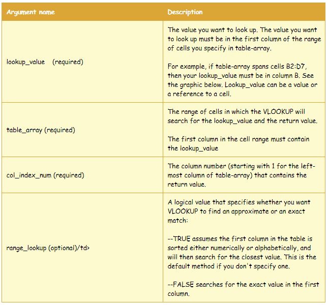
Syntax of Vlookup Function: Vlookup function have four arguments.

1. lookup_value    (required)
2. table_array    (required)
3. col_index_num    (required)
4. range_lookup   (optional)

The complete Syntax of formula is VLOOKUP (lookup_value, table_array, col_index_num, [range_lookup])

See the table below For detail understanding about the syntax of vlookup formula.

      Now you able to understand what is vlookup? and how vlookup works? And you also know about its syntax and requirements. Going forward we will do some practical exercises with real data to understand VLookup. We already know that vlookup is used for is to find a value and see whether it exists in another range of values. So I have a list of people here that Works For a company ABC, See below. So all the people that works are here in the Main data. Main data Table has three Columns. We have filled Unique Employee codes of Employees are In Column B, In Column C there is Name of Employees and in Column D Salary.


     There are two another tables (Table 2 and Table 3) are in the above-mentioned sheet. First is to find salary against of mentioned Employee Codes and second is to find Salary against the Employee name. To find the values we will use Vlookup here. According to syntax, we need to define all four arguments of Vlookup Function first. Let's start the procedure of vlookup for Table 2. 

1. lookup_value   - Lookup value will be Emp codes for Table 2 (F4, F5, F6........).
2. table_array    - Table array will be whole Table 1 (B2:D22).
3. col_index_num - Column index number for this will be 3 Because when we start counting from the First column of Table 1, salary comes on the third number. See below-attached sheet.
4. range_lookup - We will fill 0 or False here to get the exact match.

Execution of Vlookup Function :

      Now we are all set and we want to use the vlookup formula. So I'm going to click in the cell next to this first Employee Id (G4). I want to see if 89750 (F4) is part of this group. Now obviously I can see it here cuz it's a small list but when you have potentially thousands of items in your list it gets a lot more tricky to figure that out. So I'll click the insert function button and I need to use a lookup function. I can search so I'll type me look up and there's vlookup, there's lookup, H lookup. H lookup does the same thing instead of going up and down columns it goes left to right across rows. So select vlookup, and what it does the first thing it says is it explains what the function does so it  "looks for a value in the leftmost column of a table over here and then returns a  value in the same row for a column you specify". And then you notice as you click in each of these fields here to build this function it gives you an explanation, what each of them does.

Using VLOOKUP with the first Column

        So there are four fields that you need to use here. The first one is the lookup value. So what are you looking for?  You want to look up 89750 (F4) in Table 1, So cell (F4) is the lookup_value. For table_array I could drag a range of cells. So we select whole Table 1 (B2:D22). So this is where I'm going to look. I'm going to check for 89750 (F4) value and see if it's in the range (B2:D22). Then we come to column_index_number this is the column number in Table 1 that I want to return. So I have a Table that is three columns wide, if I want to find a match for this 89750 (F4) which is here do I want to return, the value in column one which is the Employee ID or in column two which is the Employee Name or in column three which in the Salary. And for this activity, I want to do an employee id, and then range_lookup, range lookup there's two options true or false. false means it has to be an exact match, true means the closest match. Most of the time you will not want to use true. You'll want an exact match. Though we use false and we're ready to go so I'll hit OK.

     So it looked for F4 value in Table 1. It found the value right there and then it returned the data. That was in the first column of the range which is the name. Now I can just drag it all the way down my range and it will look up everybody. While dragging an error appears. To avoid this error we can use two methods. First is to create a Name Range for Table 1 or second method is to freeze cells. We will learn about Naming Ranges later. We will use the second method here. For freezing cells, you can just select the table array (B2:D22) and press F4 key. After pressing F4 your selection turns like this ($B$2:$D$22), you can press F4 or you can manually put dollor $ sigh before row and column numbers. Now again drag the formula. Now it's flawless. and you are able to find all the values against the Employee Codes.

Using VLOOKUP with 2nd Column

We have just used vlookup formula with the first column in the table array. In the previous case Lookup value was in the first column. But sometimes lookup value is in the different column instead of the first column of range lookup. As shown in the below image we are going to find Salary against the employee names which in the second column of the range lookup.

In this case, Vlookup function's arguments would be as below:

1. lookup_value   - Lookup value will be Emp codes for Table 2 (F14, F15, F16........).
2. table_array    - Table array will be not the whole Table 1 this time. Table array for this case will be  (C2:C22).
3. col_index_num - Column index number for this will be 2 Because when we start counting from the second column of Table 1, salary comes on the second number. 
4. range_lookup - We will fill 0 or False here to get the exact match.

Now execute the formula according to this and follow the same procedure as we have done earlier. You will get the answer.

So we have learned using vlookup in excel. You can use vlookup function in excel 2013, and all other versions of Excel. I hope your problem has solved. Please ask me if you have any doubts or any queries via comments. Please share this article on Facebook and with your friends, this will encourage me to write more relevant tutorials for you. happy learning and thanks for reading.